---
title: "Multi-Panel Plots in R"
subtitle: "Combining and faceting figures with patchwork, cowplot, facet_wrap, and facet_grid"
author: "Noah Weidig"
date: "2026-03-28"
categories: [code, ggplot2, dataviz]
description: "Learn four powerful approaches to multi-panel plots in R — use facet_wrap and facet_grid to split a single dataset by groups, or reach for patchwork and cowplot to stitch together entirely different figures into a polished layout."
execute:
warning: false
message: false
toc: true
toc-depth: 2
code-fold: show
share:
permalink: "https://noahweidig.github.io/chartifyr/posts/multiplot/"
---
One plot is rarely enough. Whether you are comparing species across islands, aligning a scatter plot next to a box plot, or building a manuscript figure with labeled panels, multi-panel layouts are a daily tool in data visualization. R gives you two broad strategies: **faceting** (splitting one plot by a variable) and **plot composition** (gluing separate plots together). This post covers both, using the Palmer Penguins dataset throughout.
# Setup
```{r}
#| label: setup
# Uncomment to install any missing packages
# install.packages(c("ggplot2", "dplyr", "palmerpenguins", "patchwork", "cowplot"))

library(ggplot2)
library(dplyr)
library(palmerpenguins)
library(patchwork)
library(cowplot)

penguins <- palmerpenguins::penguins
```
# Faceting: Splitting One Plot by a Variable
Faceting is built into ggplot2. You write a single `ggplot()` call, then add `facet_wrap()` or `facet_grid()` to automatically replicate the plot for each level of a grouping variable. All panels share the same axes by default, making comparisons easy.
## facet_wrap
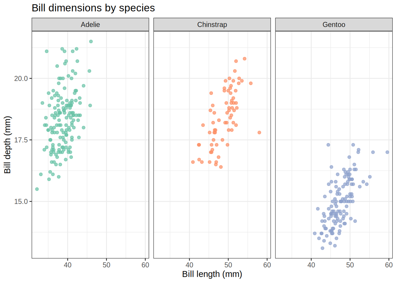
`facet_wrap()` lays panels out in a ribbon that wraps to a new row once it hits a set number of columns. It is the go-to choice when you have **one grouping variable** and want ggplot2 to handle the layout for you.
```{r}
#| label: facet-wrap-basic
ggplot(penguins, aes(x = bill_length_mm, y = bill_depth_mm, color = species)) +
  geom_point(alpha = 0.7, na.rm = TRUE) +
  facet_wrap(~species) +
  scale_color_brewer(palette = "Set2") +
  labs(
    title = "Bill dimensions by species",
    x = "Bill length (mm)",
    y = "Bill depth (mm)",
    color = "Species"
  ) +
  theme_bw() +
  theme(legend.position = "none")
```
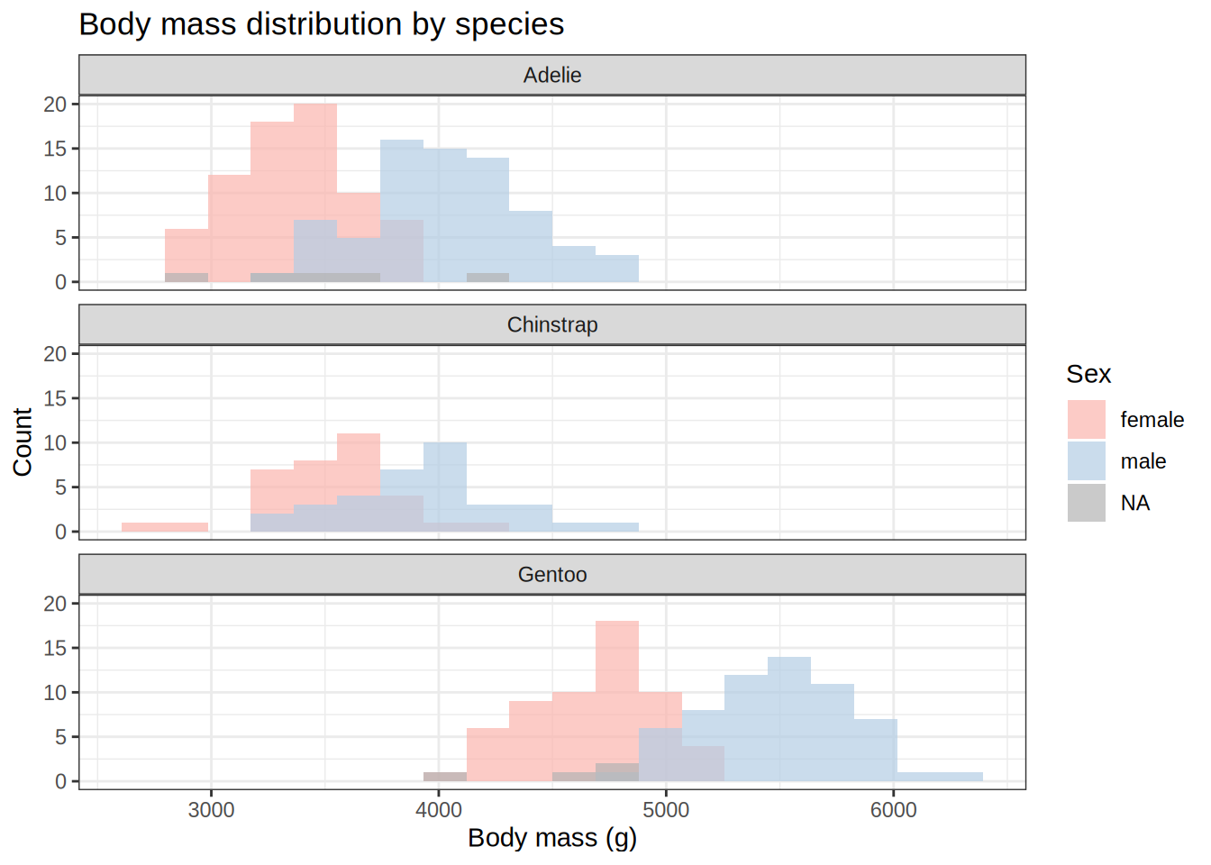
The `~species` formula tells ggplot2 which variable to facet on. By default it picks the number of columns automatically, but you can override that with `ncol` or `nrow`.
```{r}
#| label: facet-wrap-ncol
ggplot(penguins, aes(x = body_mass_g, fill = sex)) +
  geom_histogram(bins = 20, na.rm = TRUE, position = "identity", alpha = 0.7) +
  facet_wrap(~species, ncol = 1) +
  scale_fill_brewer(palette = "Pastel1", na.value = "grey70") +
  labs(
    title = "Body mass distribution by species",
    x = "Body mass (g)",
    y = "Count",
    fill = "Sex"
  ) +
  theme_bw()
```
### Free scales
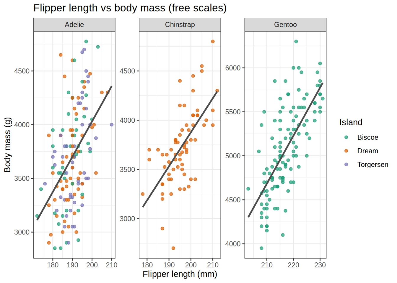
By default all panels share the same axis limits (`scales = "fixed"`). Set `scales = "free"`, `"free_x"`, or `"free_y"` when the ranges differ dramatically between groups and you care more about within-panel pattern than cross-panel comparison.
```{r}
#| label: facet-wrap-free-scales
ggplot(penguins, aes(x = flipper_length_mm, y = body_mass_g)) +
  geom_point(aes(color = island), alpha = 0.7, na.rm = TRUE) +
  geom_smooth(method = "lm", se = FALSE, na.rm = TRUE, color = "grey30") +
  facet_wrap(~species, scales = "free") +
  scale_color_brewer(palette = "Dark2") +
  labs(
    title = "Flipper length vs body mass (free scales)",
    x = "Flipper length (mm)",
    y = "Body mass (g)",
    color = "Island"
  ) +
  theme_bw()
```
## facet_grid
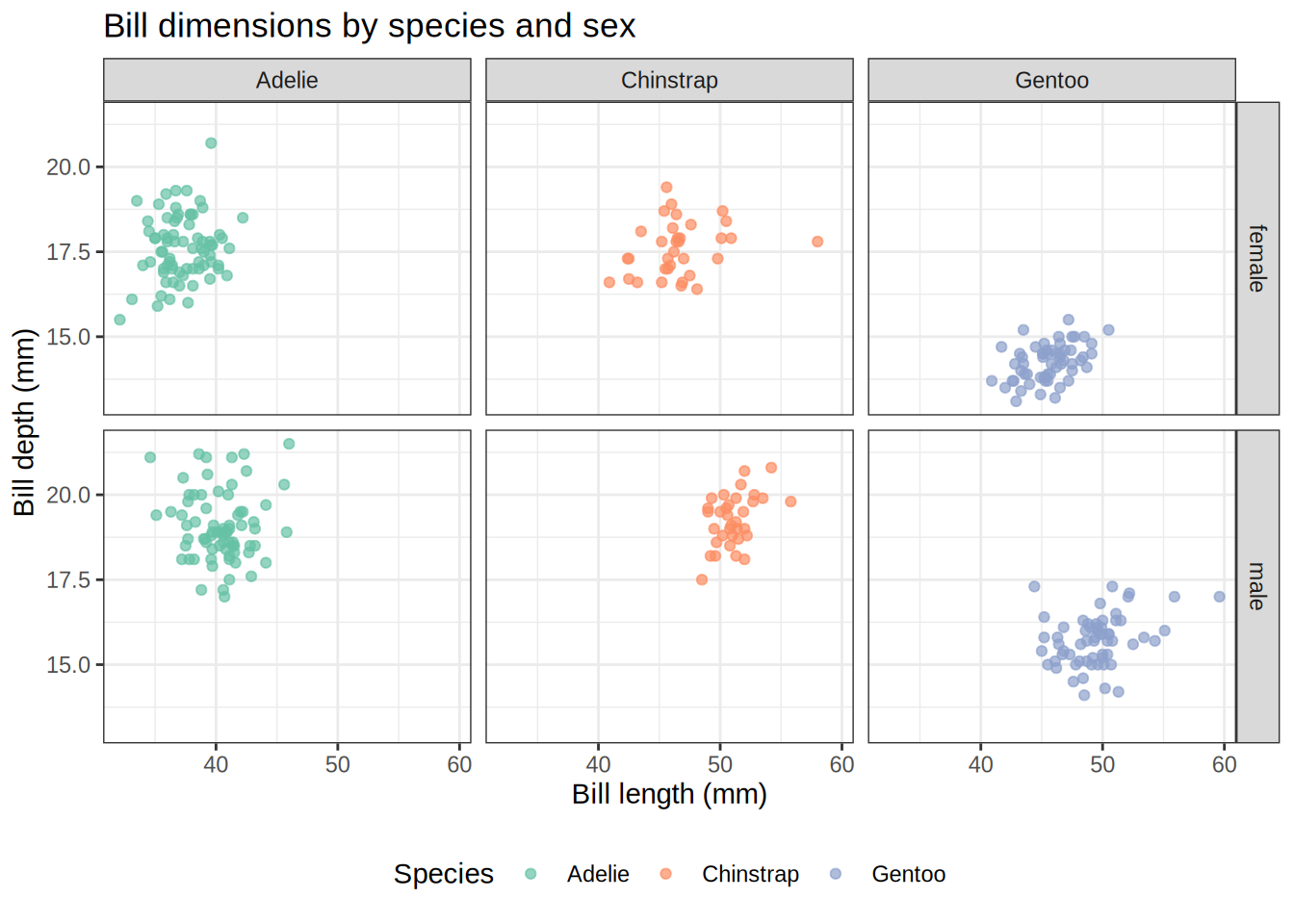
`facet_grid()` creates a strict **rows × columns** grid defined by two variables. Use it when you want to cross-tabulate two grouping variables and keep the layout perfectly aligned.
```{r}
#| label: facet-grid-basic
ggplot(
  penguins |> filter(!is.na(sex)),
  aes(x = bill_length_mm, y = bill_depth_mm)
) +
  geom_point(aes(color = species), alpha = 0.7, na.rm = TRUE) +
  facet_grid(sex ~ species) +
  scale_color_brewer(palette = "Set2") +
  labs(
    title = "Bill dimensions by species and sex",
    x = "Bill length (mm)",
    y = "Bill depth (mm)",
    color = "Species"
  ) +
  theme_bw() +
  theme(legend.position = "bottom")
```
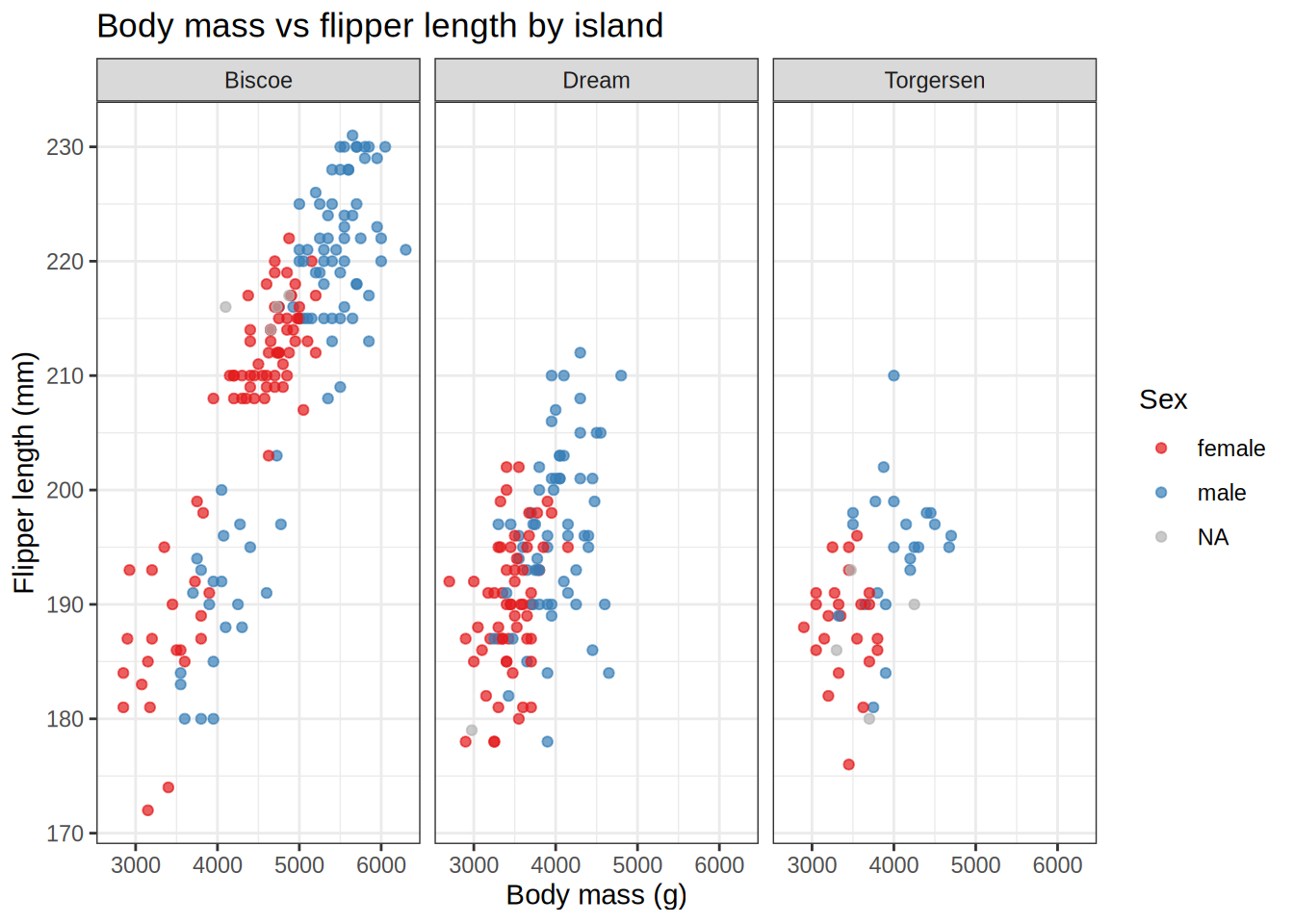
The formula `sex ~ species` puts `sex` levels along rows and `species` levels across columns. Use `.` to suppress one dimension: `~ species` gives one row of columns, `sex ~ .` gives one column of rows.
```{r}
#| label: facet-grid-one-dim
# One row of columns (equivalent to facet_wrap with fixed layout)
ggplot(penguins, aes(x = body_mass_g, y = flipper_length_mm)) +
  geom_point(aes(color = sex), alpha = 0.7, na.rm = TRUE) +
  facet_grid(. ~ island) +
  scale_color_brewer(palette = "Set1", na.value = "grey70") +
  labs(
    title = "Body mass vs flipper length by island",
    x = "Body mass (g)",
    y = "Flipper length (mm)",
    color = "Sex"
  ) +
  theme_bw()
```
### facet_wrap vs facet_grid at a glance
| Feature | `facet_wrap` | `facet_grid` |
|---|---|---|
| Variables | One | Two (rows × columns) |
| Layout | Wraps automatically | Strict grid |
| Best for | One grouping variable | Crossing two variables |
| Free scales | Yes (`scales =`) | Yes (`scales =`) |
| Space control | `nrow` / `ncol` | Fixed by variable levels |
# Plot Composition: Combining Separate Plots
Sometimes you need panels that show **different variables, geoms, or even different datasets** side by side. That is where `patchwork` and `cowplot` come in — they let you take any ggplot objects and arrange them into a single figure.
Let us build a few reusable plots to combine throughout these examples.
```{r}
#| label: base-plots
p_scatter <- ggplot(penguins, aes(x = bill_length_mm, y = bill_depth_mm,
color = species, fill = species)) +
geom_point(alpha = 0.7, na.rm = TRUE, shape = 21) +
scale_color_brewer(palette = "Set2") +
scale_fill_brewer(palette = "Set2") +
labs(x = "Bill length (mm)", y = "Bill depth (mm)", fill = "Species") +
guides(color = "none") +
theme_bw()
p_box <- ggplot(penguins, aes(x = species, y = body_mass_g, fill = species)) +
geom_boxplot(na.rm = TRUE, show.legend = FALSE) +
scale_fill_brewer(palette = "Set2") +
labs(x = "Species", y = "Body mass (g)") +
theme_bw()
p_hist <- ggplot(penguins, aes(x = flipper_length_mm, fill = species)) +
geom_histogram(bins = 25, alpha = 0.7, na.rm = TRUE, position = "identity") +
scale_fill_brewer(palette = "Set2") +
labs(x = "Flipper length (mm)", y = "Count", fill = "Species") +
theme_bw()
p_bar <- ggplot(penguins, aes(x = island, fill = species)) +
geom_bar(position = "dodge") +
scale_fill_brewer(palette = "Set2") +
labs(x = "Island", y = "Count", fill = "Species") +
theme_bw()
```
## patchwork
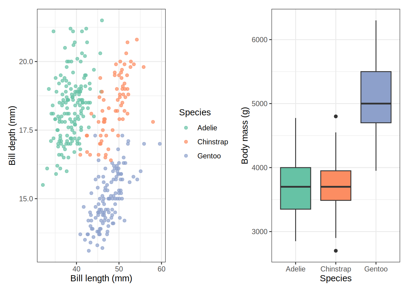
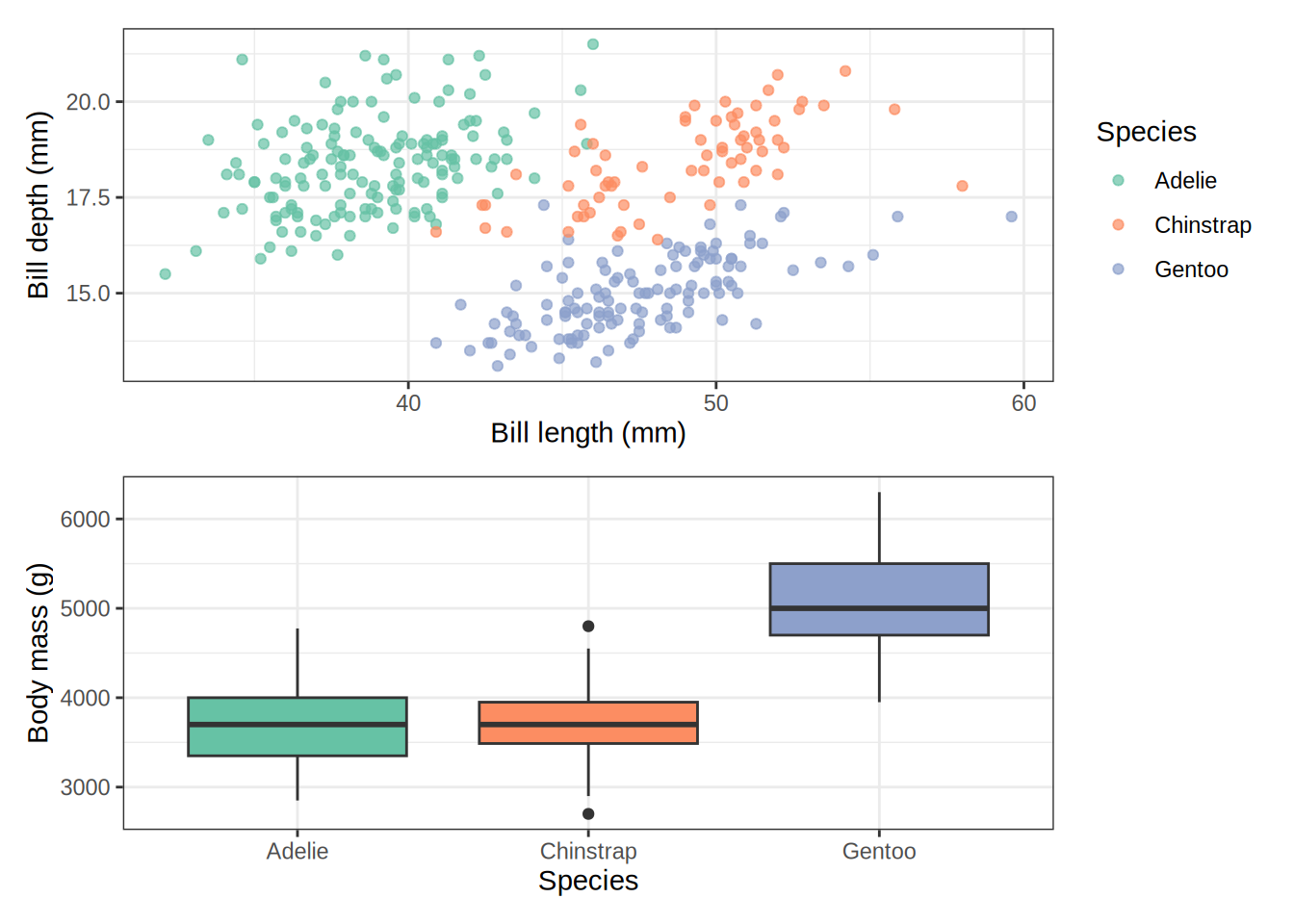
**patchwork** extends ggplot2 with a simple operator-based syntax. After loading the package, you can combine plots with `+`, `/`, and `|` exactly like arithmetic.
```{r}
#| label: patchwork-basic
# Side by side
p_scatter + p_box
```
```{r}
#| label: patchwork-stack
# Stacked
p_scatter / p_box
```
### Layouts with `plot_layout()`
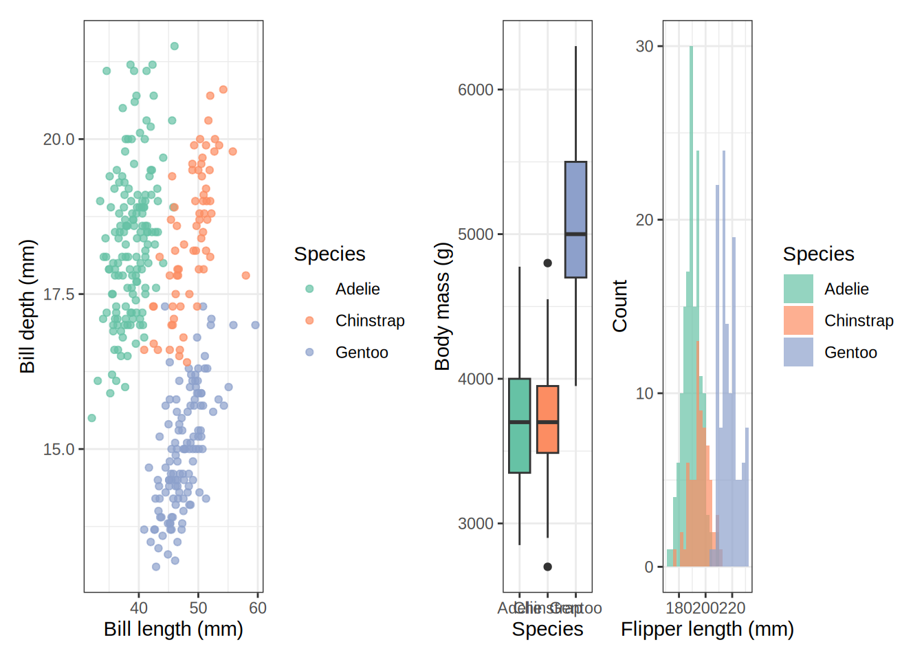
`plot_layout()` gives you fine-grained control over the grid, including relative widths, heights, and shared guides.
```{r}
#| label: patchwork-layout
(p_scatter | p_box | p_hist) +
plot_layout(widths = c(2, 1, 1), guides = "collect") &
theme(legend.position = "bottom")
```
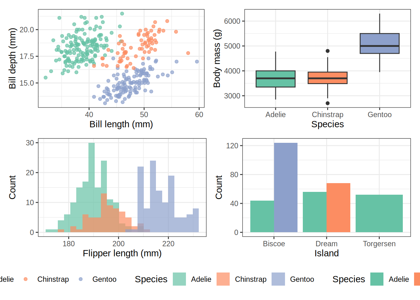
```{r}
#| label: patchwork-complex
# A 2×2 grid with shared legend collected at the bottom
(p_scatter + p_box) / (p_hist + p_bar) +
  plot_layout(guides = "collect") &
  theme(legend.position = "bottom")
```
### Panel labels with `plot_annotation()`
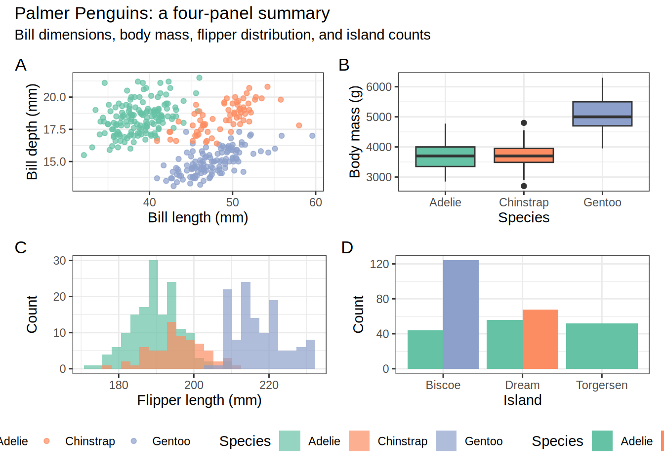
`plot_annotation()` adds a title and subtitle to the whole figure, plus automatic **A, B, C…** labels on each panel — essential for publications.
```{r}
#| label: patchwork-annotation
(p_scatter + p_box) / (p_hist + p_bar) +
  plot_annotation(
    title = "Palmer Penguins: a four-panel summary",
    subtitle = "Bill dimensions, body mass, flipper distribution, and island counts",
    tag_levels = "A"
  ) +
  plot_layout(guides = "collect") &
  theme(legend.position = "bottom")
```
### Nesting layouts
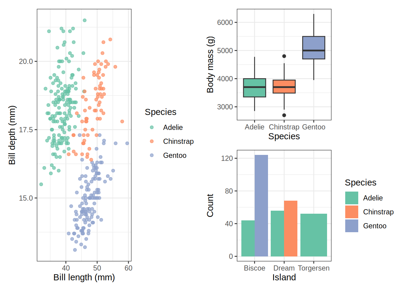
You can nest patchwork assemblies inside each other using `wrap_plots()` or by grouping with parentheses.
```{r}
#| label: patchwork-nested
right_column <- p_box / p_bar

p_scatter | right_column
```
## cowplot
**cowplot** (by Claus Wilke) takes a slightly different approach. Its main function is `plot_grid()`, which accepts a list of plots and arranges them with precise alignment control. It is especially useful when panels have different axis structures and you need **exact pixel-level alignment**.
```{r}
#| label: cowplot-basic
plot_grid(p_scatter, p_box, ncol = 2)
```
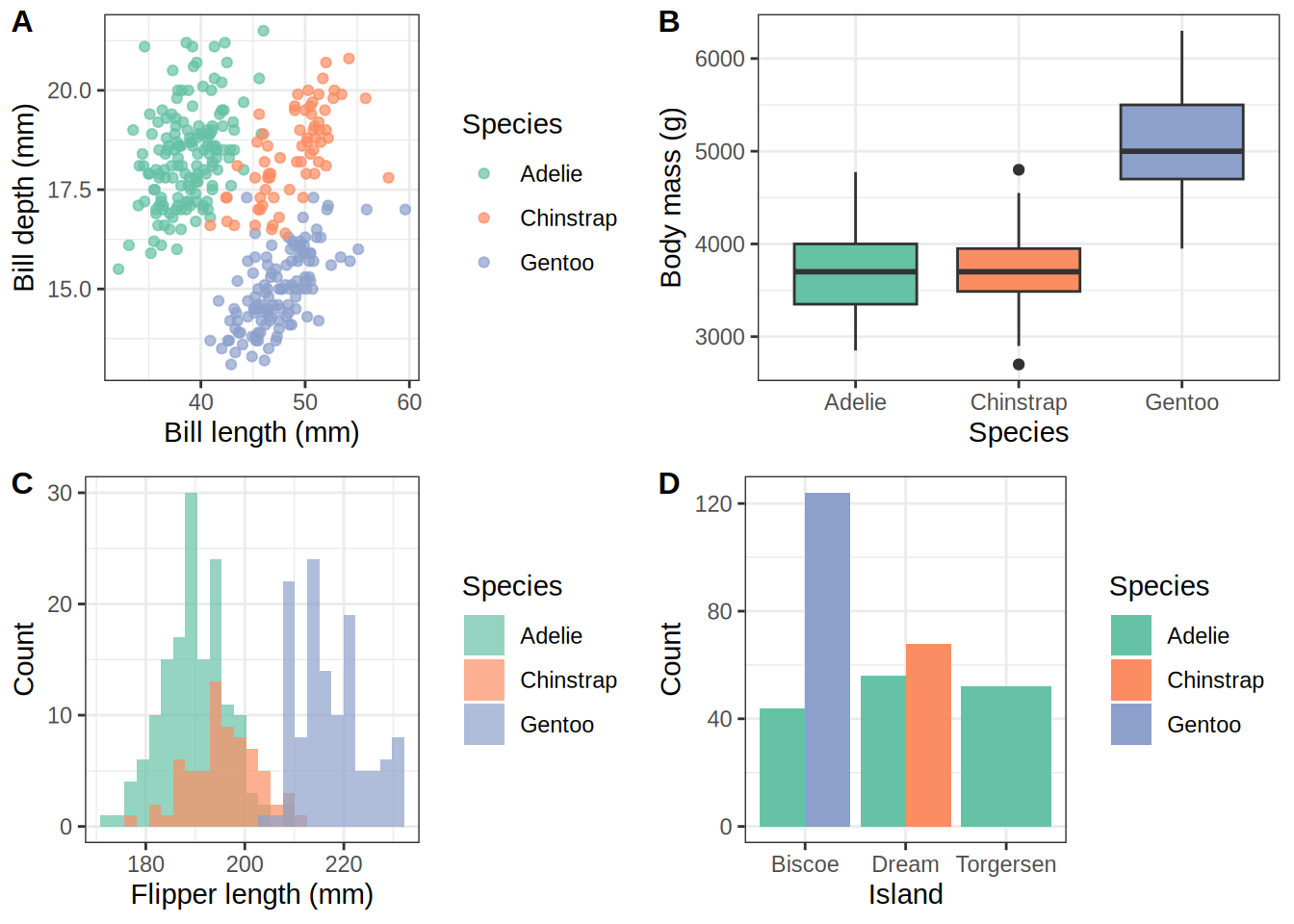
```{r}
#| label: cowplot-labels
# Add panel labels
plot_grid(p_scatter, p_box, p_hist, p_bar,
          labels = c("A", "B", "C", "D"),
          label_size = 12,
          ncol = 2)
```
### Controlling relative sizes
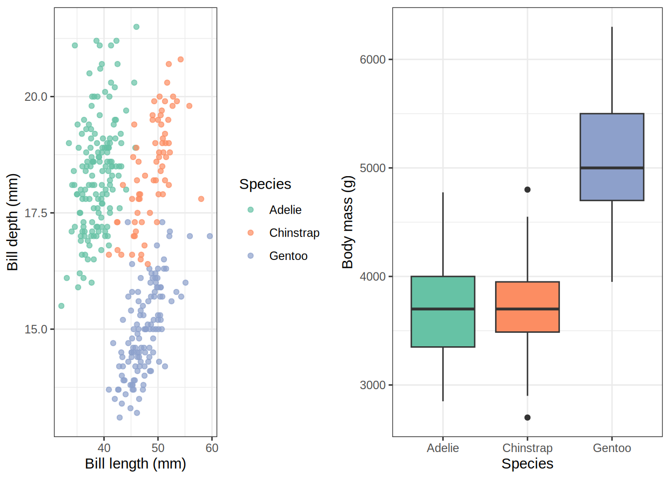
Use `rel_widths` and `rel_heights` to weight panels.
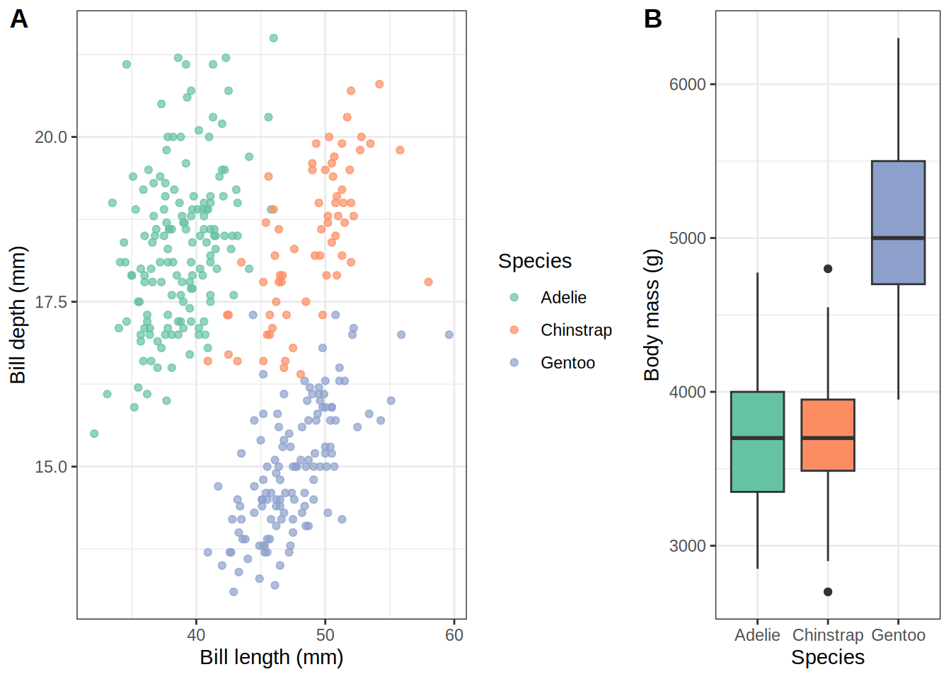
```{r}
#| label: cowplot-rel-widths
plot_grid(p_scatter, p_box,
          ncol = 2,
          rel_widths = c(2, 1),
          labels = "AUTO")
```
### Shared legends with `get_legend()`
A common cowplot pattern is to pull the legend out of one plot and place it as its own element using `get_legend()`.
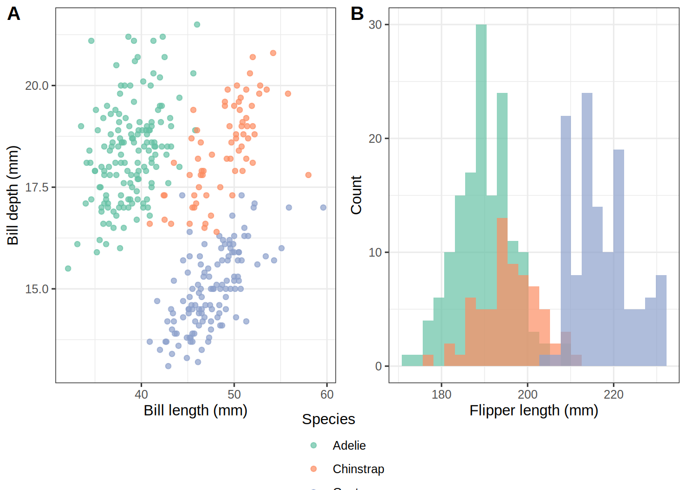
```{r}
#| label: cowplot-shared-legend
# Build plots without their own legends
p_scatter_noleg <- p_scatter + theme(legend.position = "none")
p_hist_noleg <- p_hist + theme(legend.position = "none")
# Extract legend from the original scatter
legend <- get_legend(p_scatter)
# Arrange plots + legend
top_row <- plot_grid(p_scatter_noleg, p_hist_noleg,
ncol = 2, labels = c("A", "B"))
plot_grid(top_row, legend,
ncol = 1,
rel_heights = c(1, 0.25))
```
### Aligning axes
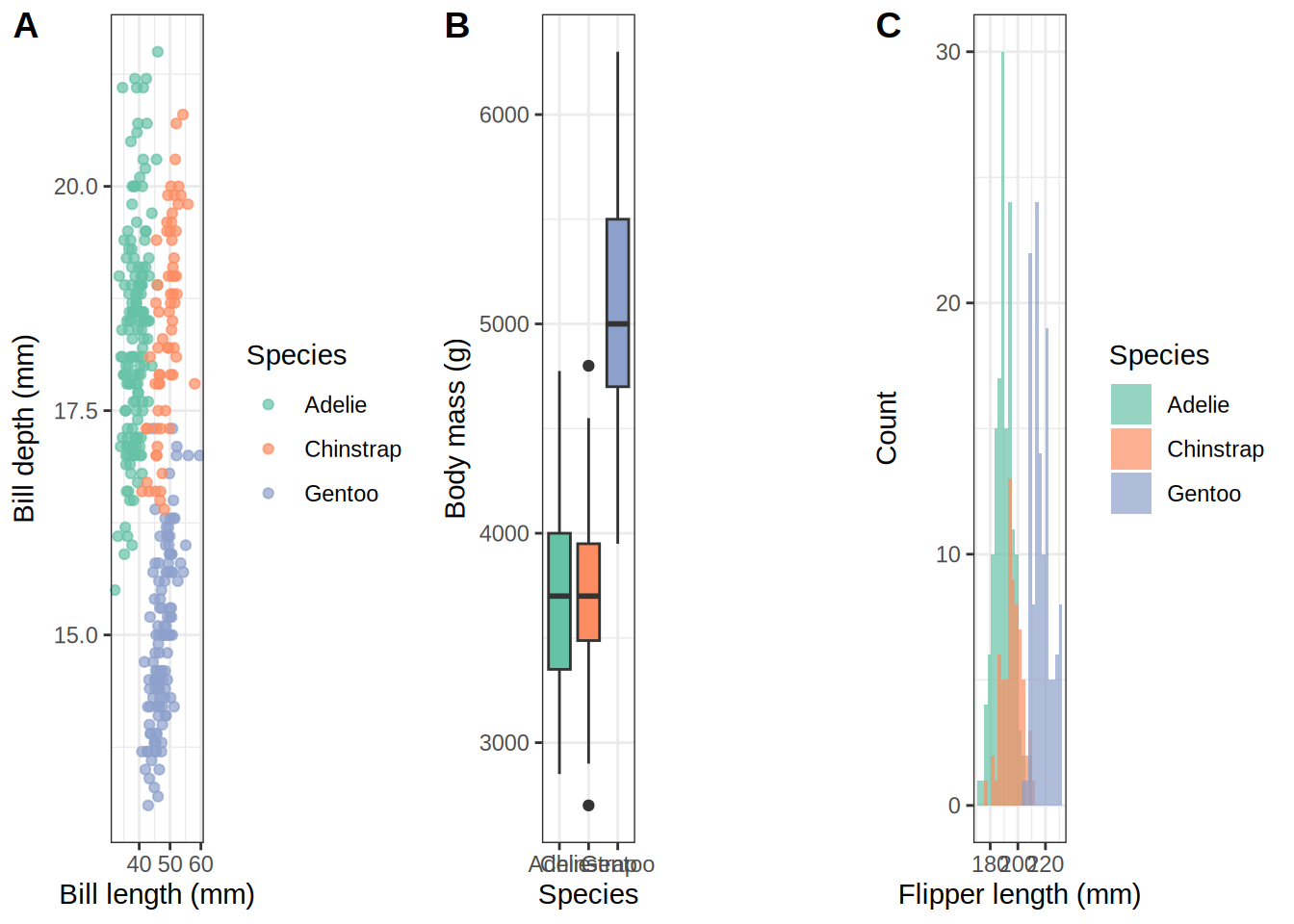
`align = "hv"` forces horizontal and vertical axis alignment across panels — critical when mixing plots with different title heights or legend sizes.
```{r}
#| label: cowplot-align
plot_grid(p_scatter + theme(legend.position = "bottom"),
p_box,
p_hist + theme(legend.position = "bottom"),
align = "hv",
ncol = 3,
labels = "AUTO")
```
## patchwork vs cowplot at a glance
| Feature | `patchwork` | `cowplot` |
|---|---|---|
| Syntax | Operators (`+`, `/`, `|`) | `plot_grid()` function |
| Learning curve | Very low | Low |
| Shared legend | `plot_layout(guides = "collect")` | `get_legend()` + `plot_grid()` |
| Axis alignment | Automatic | `align = "hv"` |
| Panel labels | `plot_annotation(tag_levels =)` | `labels =` argument |
| Nesting | Parentheses / `wrap_plots()` | Nested `plot_grid()` calls |
| Best for | Quick layouts, publications | Precise alignment, mixed axes |
# Putting It All Together
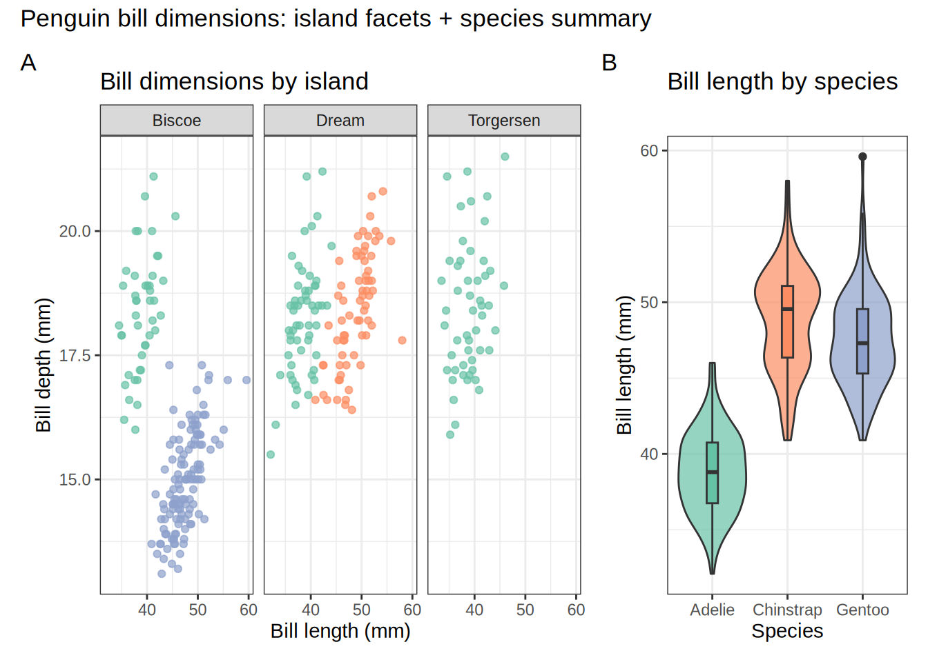
You can even combine faceting *and* composition. Here we facet a scatter plot by island, then place it alongside a summary box plot.
```{r}
#| label: combined
p_faceted <- ggplot(penguins, aes(x = bill_length_mm, y = bill_depth_mm,
                                   color = species)) +
  geom_point(alpha = 0.7, na.rm = TRUE) +
  facet_wrap(~island) +
  scale_color_brewer(palette = "Set2") +
  labs(
    title = "Bill dimensions by island",
    x = "Bill length (mm)",
    y = "Bill depth (mm)",
    color = "Species"
  ) +
  theme_bw() +
  theme(legend.position = "none")

p_summary <- ggplot(penguins, aes(x = species, y = bill_length_mm,
                                   fill = species)) +
  geom_violin(na.rm = TRUE, alpha = 0.7, show.legend = FALSE) +
  geom_boxplot(width = 0.15, na.rm = TRUE, show.legend = FALSE) +
  scale_fill_brewer(palette = "Set2") +
  labs(
    title = "Bill length by species",
    x = "Species",
    y = "Bill length (mm)"
  ) +
  theme_bw()

p_faceted + p_summary +
  plot_layout(widths = c(2, 1)) +
  plot_annotation(
    title   = "Penguin bill dimensions: island facets + species summary",
    tag_levels = "A"
  )
```
# Quick Reference
| Goal | Tool | Key argument |
|---|---|---|
| Split one plot by one variable | `facet_wrap(~var)` | `ncol`, `nrow`, `scales` |
| Cross two grouping variables | `facet_grid(r ~ c)` | `scales`, `space` |
| Place plots side by side | `p1 \| p2` (patchwork) | — |
| Stack plots vertically | `p1 / p2` (patchwork) | — |
| Control widths/heights | `plot_layout()` | `widths`, `heights` |
| Add figure title + labels | `plot_annotation()` | `title`, `tag_levels` |
| Arrange with precise alignment | `plot_grid()` (cowplot) | `align`, `rel_widths` |
| Shared legend (cowplot) | `get_legend()` | — |
Multi-panel layouts take a little practice, but once you have the patterns down they become second nature. Start with `facet_wrap` whenever a single variable is doing the grouping, reach for `facet_grid` when you are crossing two factors, and pull in `patchwork` or `cowplot` whenever you need to combine fundamentally different plots into one cohesive figure.